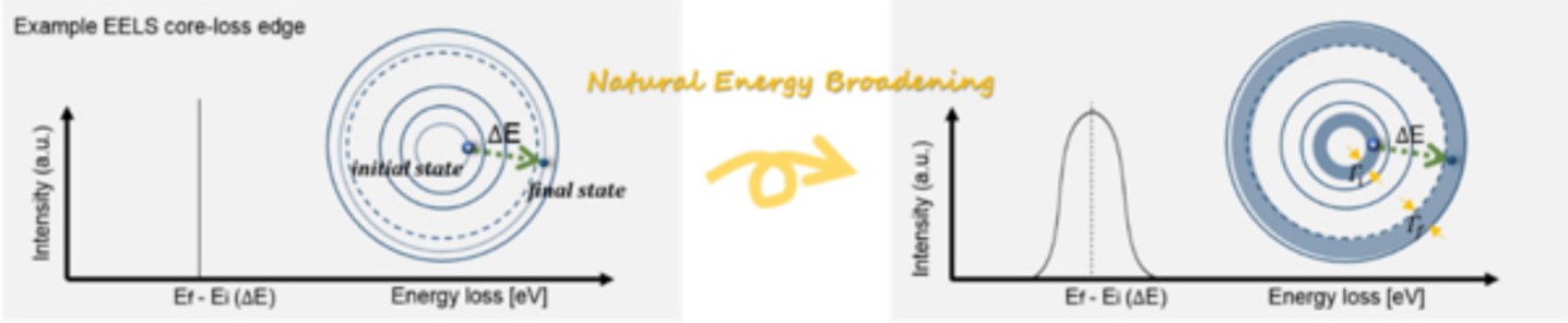
Natural Energy Broadening

Core-loss edges in EELS are generated due to the excitation of core electrons to the empty energy level above the Fermi energy. The initial (i) and final (f) states of the excitation have uncertainties in their energy due to a finite lifetime. (Heisenberg uncertainty principle) The uncertainty in the energy induces the energy broadening of each state, which is referred to as the energy level width Γ.

Links:
Github
FileExchange

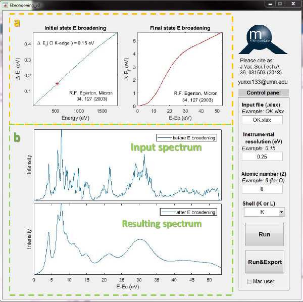
In this code, the energy broadening of the initial and the final state is implemented to a simulated EELS spectrum. The energy level width of the initial state, Γi, is relatively small and almost constant for a chosen core-loss edge. (See the left box of (a)) The energy level width of the final state, Γf, is relatively big (0~6 eV) and varies with the final energy relative to the onset energy of core-loss edge. (See the right box of (a)) The input EELS data is convolved with Lorentzian function with the FWHM of Γi and Γf, consecutively. The example input and resulting EELS spectra are shown in (b).

STEM EDX Data Fitting

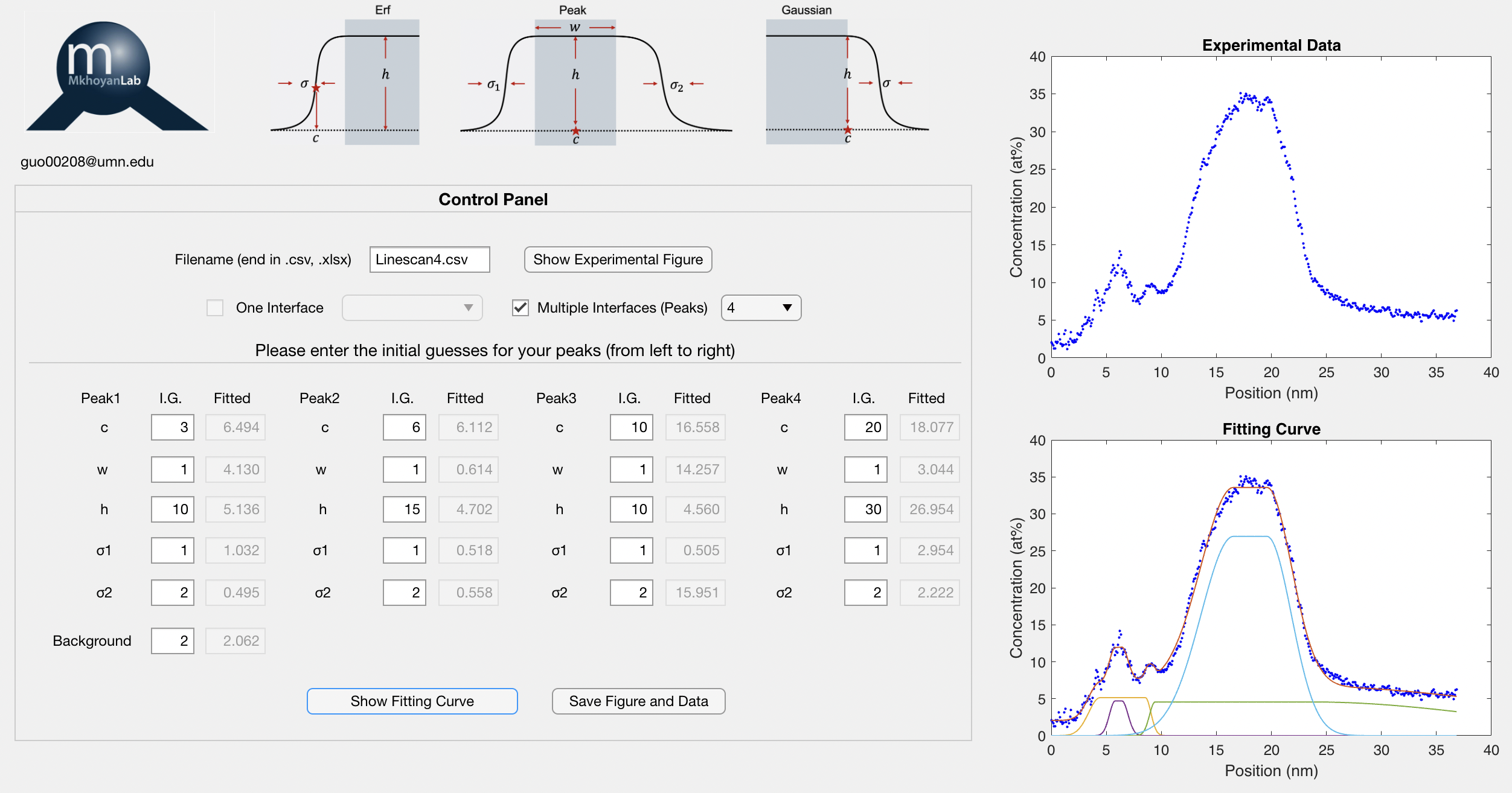
Energy dispersive X-ray spectrum (EDX) data are obtained using (scanning) transmission electron microscopy (STEM) to study the compositional information of functional layers in nano scale electronic devices. In particular, electronic devices such as transistors and memristors are consisted of multiple functional layers, resulting in several interfaces between nano-meter thick materials. To study the influence of materials distribution and diffusion at the interface, it is critical to fit the multi-peak EDX data with precise piecewise functions.
Links:
Github

Here we built an EDX fitting APP (in MATLAB®) with customized Gaussian-platform piecewise functions to discover underlying parameters of the EDX data, using first-choice local search algorithms with user-defined restart. Due to different number of interfaces in the electronic devices, the EDX data usually presents different shapes (one to four peaks, sometimes with platform functions). Therefore, this Matlab app provides several options:

• One interface: Erf (error function), Erfc (complementary error function), left Gaussian and right Gaussian
• Multiple interfaces: 1 peak, 2 peaks, 3 peaks, 4 peaks

Users can choose different fitting functions according to the shape of their EDX data.

Installation

To install this app in your MATLAB®:

1. Make sure that the MATLAB® - Curve Fitting Toolbox is already installed.
2. Copy the STEM EDX Fitting.mlappinstall file to your current working folder in
MATLAB®.
3. Right click on the file and select ‘Install’

Usage

Users need to put initial starting points for parameters of their EDX data. For examples, the parameters (c, w, h, σ1, σ2) for every peak are defined in the following images.

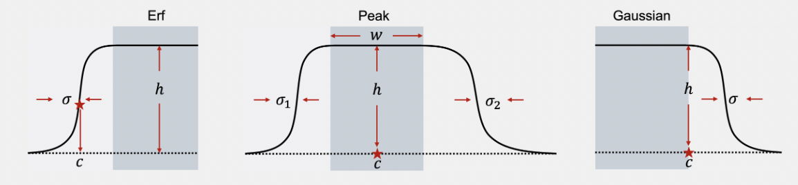
After type in the initial guess of platform positions, widths, heights and standard deviations, click Show Fitting Curve button to start the fitting progress. Note that the more platforms the EDX data has, the longer it takes to perform the fitting due to increase of parameters. Users can also adjust the starting point to get better fitting results.

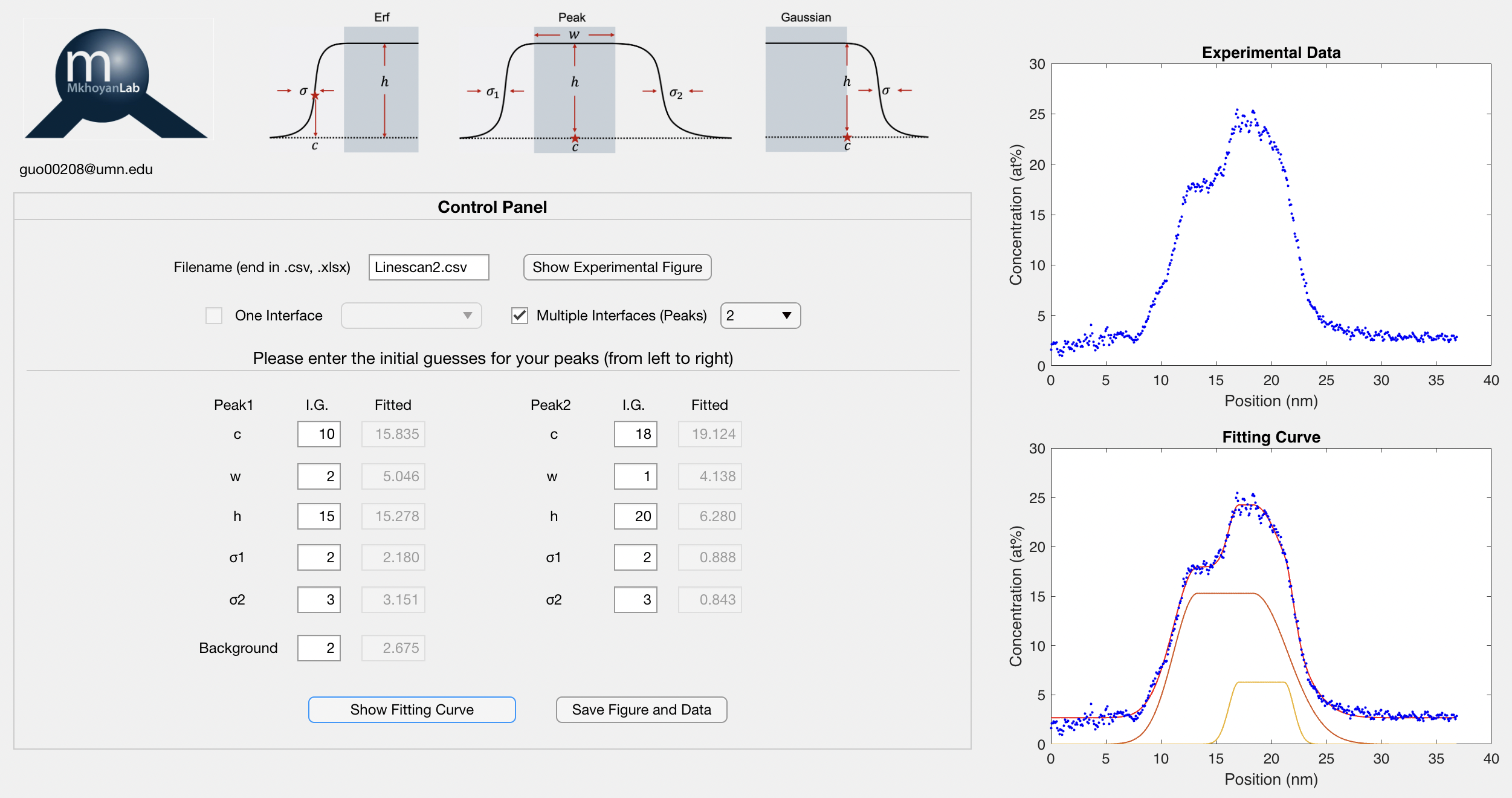
Here are two examples of two-platform data fitting and four-platform data fitting:
1. Two-Platforms Fitting

2. Four-Platforms Fitting

Finally, click the Save Figure and Data button to save the fitted data, fitted parameters, and figures to the same folder

Citation

Please cite this code if used for publication purpose:
Guo, S. STEM EDX Data Fitting. (2023) Retrieved from (https://github.com/siluguo/STEM-
EDX-Data-Fitting)